
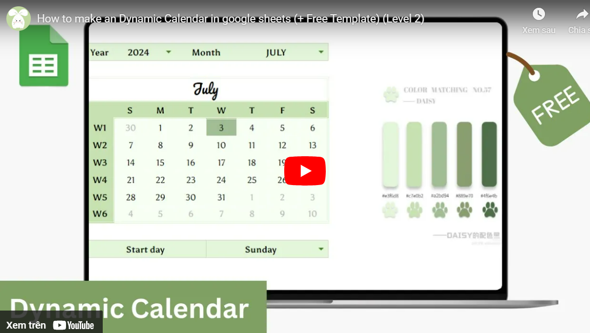
Today, I’ll guide you step-by-step on how to create a dynamic calendar in level 2 Google Sheets. With this calendar, you can select the start day of the week, and today’s date will be automatically highlighted. I’ve also used this calendar in my content planner, and it’s been a game-changer. Let’s get started!
Step 1: Set Up Your Spreadsheet
Open a new Google Sheets file.
Resize the columns and rows to create a neat and compact calendar layout.
Align the text:
Horizontal alignment: Center.
Vertical alignment: Middle.
Enable text wrapping: Wrap.
Use the Border function to outline the calendar grid.
Step 2: Create the Grid for Dates
Design a grid with enough space to display all the days of the month (6 rows for weeks and 7 columns for days).
Label the second row with the initials of the weekdays (e.g., Mon, Tue, etc.).
Step 3: Add Drop-Down Menus for Year and Month
Create a new sheet and name it “Setup”.
In the “Setup” sheet, list the years and months you want to include.
Go back to the main sheet, click Insert > Drop-Down, and select the range from the “Setup” sheet.
Repeat this process for both the year and month dropdown menus.
Pro Tip: This setup allows you to update the calendar by simply changing the year or month in the dropdown menu.
Step 4: Display the Selected Month and Year
Use the formula
=DATE(year, month, 1)to create a reference date.Format the display using Format > Number > Custom date and time, and choose your preferred format (e.g., “Month YYYY”).
Step 5: Select the Start Day of the Week
Add a drop-down menu to select the start day (e.g., Sunday or Monday).
For simplicity, directly input the options into the drop-down setup without referencing the “Setup” sheet.
Step 6: Generate the Weekdays Automatically
Use the formula
=TEXT(date, "ddd")to dynamically display weekdays based on the selected start day.
Step 7: Add Week Numbers
Label the leftmost column with “W1, W2, W3,…” up to “W6”.
Add additional rows if necessary to accommodate all weeks.
Step 8: Fill in the Days of the Month
Use the formula
=SEQUENCE(6, 7, start_date, 1)to generate the dates for the calendar.Use conditional formatting to:
Turn days that don’t belong to the current month gray.
Highlight today’s date.
Example formula for conditional formatting:
For non-current month days:
=MONTH(cell)<>MONTH(reference_month).For today’s date:
=cell=TODAY().
Step 9: Customize Your Calendar
Remove all default borders.
Choose a color palette:
Search “color palette [your preferred color]” on Pinterest for inspiration.
Use the Color Picker to match your desired theme.
Change the font style to make your calendar visually appealing.
Get the Free Template
Thank you for following along! If you found this tutorial helpful, please like this post, it is a motivation for me to write more blogs about this topic. Have a wonderful day!